ディープラーニングの畳み込みニューラルネットワーク（CNN）の中間層の出力を可視化してみました。可視化に使用したのは、５種類の花の分類に使用したVGG16を転移学習したモデルです。VGG16は、ディープラーニングによる画像応用の代表的なモデルの一つです。

VGG16（転移学習）モデルの中間層を可視化してみる。

In [1]:

import os

import keras
from keras.preprocessing.image import ImageDataGenerator
from keras.models import Sequential, Model
from keras.layers import Input, Dense, Dropout, Activation, Flatten
from keras import optimizers
from keras.applications.vgg16 import VGG16

Using TensorFlow backend.

In [2]:

keras.__version__

Out[2]:

'2.2.4'

訓練画像、検証画像、テスト画像のディレクトリ

In [3]:

# 分類クラス
classes = ['daisy', 'dandelion','rose','sunflower','tulip']
nb_classes = len(classes)
batch_size_for_data_generator = 20

base_dir = "."

test_dir = os.path.join(base_dir, 'test_images')

test_daisy_dir = os.path.join(test_dir, 'daisy')
test_dandelion_dir = os.path.join(test_dir, 'dandelion')
test_rose_dir = os.path.join(test_dir, 'rose')
test_sunflower_dir = os.path.join(test_dir, 'sunflower')
test_tulip_dir = os.path.join(test_dir, 'tulip')

# 画像サイズ
img_rows, img_cols = 200, 200

VGG16モデル

In [4]:

input_tensor = Input(shape=(img_rows, img_cols, 3))
vgg16 = VGG16(include_top=False, weights='imagenet', input_tensor=input_tensor)
#vgg16.summary()

VGG16モデルに全結合分類器を追加する

In [5]:

top_model = Sequential()
top_model.add(Flatten(input_shape=vgg16.output_shape[1:]))
top_model.add(Dense(256, activation='relu'))
top_model.add(Dropout(0.5))
top_model.add(Dense(nb_classes, activation='softmax'))
model = Model(inputs=vgg16.input, outputs=top_model(vgg16.output))
model.summary()

_________________________________________________________________
Layer (type)                 Output Shape              Param #   
=================================================================
input_1 (InputLayer)         (None, 200, 200, 3)       0         
_________________________________________________________________
block1_conv1 (Conv2D)        (None, 200, 200, 64)      1792      
_________________________________________________________________
block1_conv2 (Conv2D)        (None, 200, 200, 64)      36928     
_________________________________________________________________
block1_pool (MaxPooling2D)   (None, 100, 100, 64)      0         
_________________________________________________________________
block2_conv1 (Conv2D)        (None, 100, 100, 128)     73856     
_________________________________________________________________
block2_conv2 (Conv2D)        (None, 100, 100, 128)     147584    
_________________________________________________________________
block2_pool (MaxPooling2D)   (None, 50, 50, 128)       0         
_________________________________________________________________
block3_conv1 (Conv2D)        (None, 50, 50, 256)       295168    
_________________________________________________________________
block3_conv2 (Conv2D)        (None, 50, 50, 256)       590080    
_________________________________________________________________
block3_conv3 (Conv2D)        (None, 50, 50, 256)       590080    
_________________________________________________________________
block3_pool (MaxPooling2D)   (None, 25, 25, 256)       0         
_________________________________________________________________
block4_conv1 (Conv2D)        (None, 25, 25, 512)       1180160   
_________________________________________________________________
block4_conv2 (Conv2D)        (None, 25, 25, 512)       2359808   
_________________________________________________________________
block4_conv3 (Conv2D)        (None, 25, 25, 512)       2359808   
_________________________________________________________________
block4_pool (MaxPooling2D)   (None, 12, 12, 512)       0         
_________________________________________________________________
block5_conv1 (Conv2D)        (None, 12, 12, 512)       2359808   
_________________________________________________________________
block5_conv2 (Conv2D)        (None, 12, 12, 512)       2359808   
_________________________________________________________________
block5_conv3 (Conv2D)        (None, 12, 12, 512)       2359808   
_________________________________________________________________
block5_pool (MaxPooling2D)   (None, 6, 6, 512)         0         
_________________________________________________________________
sequential_1 (Sequential)    (None, 5)                 4720133   
=================================================================
Total params: 19,434,821
Trainable params: 19,434,821
Non-trainable params: 0
_________________________________________________________________

In [6]:

model.compile(loss='categorical_crossentropy',optimizer=optimizers.RMSprop(lr=1e-5), metrics=['acc'])

学習結果を読み出す

In [7]:

hdf5_file = os.path.join(base_dir, 'flower-model.hdf5')
model.load_weights(hdf5_file)

In [8]:

import matplotlib.pyplot as plt

In [9]:

%matplotlib inline

実際にテスト画像を分離してみる

In [10]:

import numpy as np
from keras.preprocessing.image import load_img, img_to_array
from keras.applications.vgg16 import preprocess_input

In [11]:

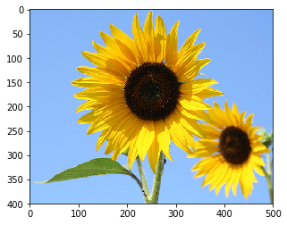
filename = os.path.join(test_dir, 'sunflower')
filename = os.path.join(filename, '3681233294_4f06cd8903.jpg')
filename

Out[11]:

'.\\test_images\\sunflower\\3681233294_4f06cd8903.jpg'

In [12]:

from PIL import Image

In [13]:

img = np.array( Image.open(filename))
plt.imshow( img )

Out[13]:

<matplotlib.image.AxesImage at 0x1f04ab81588>

テストデータ

In [14]:

img = load_img(filename, target_size=(img_rows, img_cols))
x = img_to_array(img)
x = np.expand_dims(x, axis=0)

predict = model.predict(preprocess_input(x))
for pre in predict:
    y = pre.argmax()
    print("test result=",classes[y], pre)

test result= sunflower [0.01896895 0.         0.         0.98103106 0.        ]

出力する中間層を選択する

In [15]:

layer_outputs = [layer.output for layer in model.layers[2:19]]
layer_outputs

Out[15]:

[<tf.Tensor 'block1_conv2/Relu:0' shape=(?, 200, 200, 64) dtype=float32>,
 <tf.Tensor 'block1_pool/MaxPool:0' shape=(?, 100, 100, 64) dtype=float32>,
 <tf.Tensor 'block2_conv1/Relu:0' shape=(?, 100, 100, 128) dtype=float32>,
 <tf.Tensor 'block2_conv2/Relu:0' shape=(?, 100, 100, 128) dtype=float32>,
 <tf.Tensor 'block2_pool/MaxPool:0' shape=(?, 50, 50, 128) dtype=float32>,
 <tf.Tensor 'block3_conv1/Relu:0' shape=(?, 50, 50, 256) dtype=float32>,
 <tf.Tensor 'block3_conv2/Relu:0' shape=(?, 50, 50, 256) dtype=float32>,
 <tf.Tensor 'block3_conv3/Relu:0' shape=(?, 50, 50, 256) dtype=float32>,
 <tf.Tensor 'block3_pool/MaxPool:0' shape=(?, 25, 25, 256) dtype=float32>,
 <tf.Tensor 'block4_conv1/Relu:0' shape=(?, 25, 25, 512) dtype=float32>,
 <tf.Tensor 'block4_conv2/Relu:0' shape=(?, 25, 25, 512) dtype=float32>,
 <tf.Tensor 'block4_conv3/Relu:0' shape=(?, 25, 25, 512) dtype=float32>,
 <tf.Tensor 'block4_pool/MaxPool:0' shape=(?, 12, 12, 512) dtype=float32>,
 <tf.Tensor 'block5_conv1/Relu:0' shape=(?, 12, 12, 512) dtype=float32>,
 <tf.Tensor 'block5_conv2/Relu:0' shape=(?, 12, 12, 512) dtype=float32>,
 <tf.Tensor 'block5_conv3/Relu:0' shape=(?, 12, 12, 512) dtype=float32>,
 <tf.Tensor 'block5_pool/MaxPool:0' shape=(?, 6, 6, 512) dtype=float32>]

中間層を出力するモデルを作成する

In [16]:

activation_model = Model(inputs=model.input, outputs=layer_outputs)
activation_model.summary()

_________________________________________________________________
Layer (type)                 Output Shape              Param #   
=================================================================
input_1 (InputLayer)         (None, 200, 200, 3)       0         
_________________________________________________________________
block1_conv1 (Conv2D)        (None, 200, 200, 64)      1792      
_________________________________________________________________
block1_conv2 (Conv2D)        (None, 200, 200, 64)      36928     
_________________________________________________________________
block1_pool (MaxPooling2D)   (None, 100, 100, 64)      0         
_________________________________________________________________
block2_conv1 (Conv2D)        (None, 100, 100, 128)     73856     
_________________________________________________________________
block2_conv2 (Conv2D)        (None, 100, 100, 128)     147584    
_________________________________________________________________
block2_pool (MaxPooling2D)   (None, 50, 50, 128)       0         
_________________________________________________________________
block3_conv1 (Conv2D)        (None, 50, 50, 256)       295168    
_________________________________________________________________
block3_conv2 (Conv2D)        (None, 50, 50, 256)       590080    
_________________________________________________________________
block3_conv3 (Conv2D)        (None, 50, 50, 256)       590080    
_________________________________________________________________
block3_pool (MaxPooling2D)   (None, 25, 25, 256)       0         
_________________________________________________________________
block4_conv1 (Conv2D)        (None, 25, 25, 512)       1180160   
_________________________________________________________________
block4_conv2 (Conv2D)        (None, 25, 25, 512)       2359808   
_________________________________________________________________
block4_conv3 (Conv2D)        (None, 25, 25, 512)       2359808   
_________________________________________________________________
block4_pool (MaxPooling2D)   (None, 12, 12, 512)       0         
_________________________________________________________________
block5_conv1 (Conv2D)        (None, 12, 12, 512)       2359808   
_________________________________________________________________
block5_conv2 (Conv2D)        (None, 12, 12, 512)       2359808   
_________________________________________________________________
block5_conv3 (Conv2D)        (None, 12, 12, 512)       2359808   
_________________________________________________________________
block5_pool (MaxPooling2D)   (None, 6, 6, 512)         0         
=================================================================
Total params: 14,714,688
Trainable params: 14,714,688
Non-trainable params: 0
_________________________________________________________________

入力画像を確認する

In [17]:

img = load_img(filename, target_size=(img_rows, img_cols))
x = img_to_array(img)
x = np.expand_dims(x, axis=0)
img_tensor = x/255.
print(img_tensor.shape)

(1, 200, 200, 3)

In [18]:

plt.imshow(img_tensor[0])
plt.show()

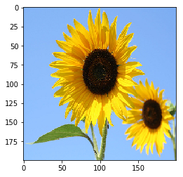
テストデータ

中間層を出力するモデルの予測を実行する

In [19]:

activations = activation_model.predict(img_tensor)

In [20]:

print(len(activations))
print(activations)

17
[array([[[[6.800552  , 0.57093966, 0.        , ..., 2.1027896 ,
          5.107834  , 1.7228966 ],
         [1.9341383 , 0.6839378 , 0.        , ..., 3.701858  ,
          2.9563394 , 1.1844163 ],
         [2.320161  , 0.7169864 , 0.        , ..., 3.57191   ,
          1.5985914 , 0.6104782 ],
         ...,


途中省略

         [0.59270453, 0.        , 0.        , ..., 0.06857053,
          0.81897503, 0.        ],
         [0.43564817, 0.        , 0.        , ..., 0.        ,
          0.86589926, 0.        ],
         [0.        , 0.        , 0.        , ..., 0.        ,
          0.7615276 , 0.        ],
         [0.        , 0.        , 0.        , ..., 0.        ,
          0.        , 0.        ]]]], dtype=float32)]

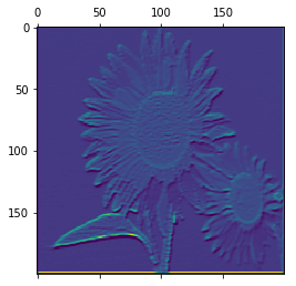
最初の畳み込み層の活性化を可視化する（一部チャンネルのみ）

In [21]:

first_layer_activation = activations[0]
print(first_layer_activation.shape)

(1, 200, 200, 64)

In [22]:

plt.matshow(first_layer_activation[0, :, :, 4], cmap='viridis')
plt.show()

最初の畳み込み層の出力（4ch）

In [23]:

plt.matshow(first_layer_activation[0, :, :, 63], cmap='viridis')
plt.show()

最初の畳み込み層の出力（63ch）

最後の畳み込み層の活性化を可視化する（一部チャンネルのみ）

In [24]:

last_layer_activation = activations[16]
print(last_layer_activation.shape)

(1, 6, 6, 512)

In [25]:

plt.matshow(last_layer_activation[0, :, :, 0], cmap='viridis')
plt.show()

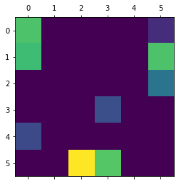
最後の畳み込み層（0ch）の出力

In [26]:

plt.matshow(last_layer_activation[0, :, :, 510], cmap='viridis')
plt.show()

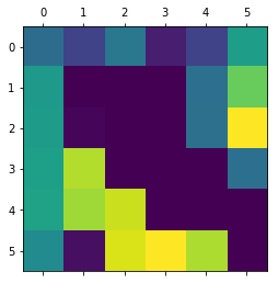
最後の畳み込み層（510ch）の出力

＜参考＞
Francois Chollet 著、株式会社クイープ翻訳、巣籠悠輔監訳、「PythonとKerasによるディープラーニング」、マイナビ出版